a := matrix([ax,ay]):
b := matrix([bx,by]):
c := matrix([cx,cy]):a,b,c
Vektorraum erkunden
Prof. Dr. Dörte Haftendorn, MuPAD 4, https://mathe.web.leuphana.de Aug.06
Automatische Übersetzung aus MuPAD 3.11, Mrz 06 Update 14.03.06
Es fehlen noch textliche Änderungen, die MuPAD 4 direkt berücksichtigen, das ist in Arbeit.
Web: https://mathe.web.leuphana.de www.mathematik-verstehen.de
+++++++++++++++++++++++++++++++++++++++++++++++++++++++++++++++++++++
1. Vektorraum und seine Gesetze (in 2D)
2. Vektoren 2D visualisieren
3. Vektoren 3D visualisieren
4. Vektorraumgesetze 3D visualisieren
###########################################
1. Vektorraum und seine Gesetze (in 2D)
-------------------------------------------------------------------------------
Vektoren werden als Matrizen aufgefasst.
Eingabe einer "flachen" Liste erzeugt Spaltenvektoren.
a := matrix([ax,ay]):
b := matrix([bx,by]):
c := matrix([cx,cy]):a,b,c
Nun gelten alle VR-Gesetze
a+b
a+(b+c)=a+(b+c)
ai:=-a

o:=a+ai

b+o

V={a,b,x,o,....} ist mit + eine Gruppe
s*a

bool(1*a=a)
![]()
Dist1:=(r*(a+b)=r*a+r*b)
expand(Dist1)
bool(expand(Dist1))
![]()
Dist2:=((r+s)*a=r*a+s*a)
bool(expand(Dist2))
![]()
r*(s*a)=(r*s)*a
(V,+) bildet mit der Skalaren-Multiplikation einen VR
a,b,r,s
#############################################
2. Vektoren 2D visualisieren
----------------------------------------------------------------------------------
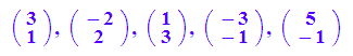
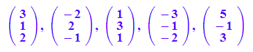
a := matrix([3,1]);
b := matrix([-2,2]);


a,b,a+b,-a,a-b
av:=plot::Arrow2d(a):
bv:=plot::Arrow2d(b):
apb:=plot::Arrow2d(a+b):
ai:=plot::Arrow2d(-a):
amb:=plot::Arrow2d(a-b):
plot(av,bv,apb,ai,amb)
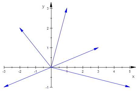
So kann man nicht erkennen, welches welcher Vektor ist.
(Nette Aufgabe!)
av:=plot::Arrow2d(a,LineColor=RGB::Green):
bv:=plot::Arrow2d(b,LineColor=RGB::Blue):
apb:=plot::Arrow2d(a+b,LineColor=RGB::Red):
ai:=plot::Arrow2d(-a,LineColor=RGB::Maroon):
amb:=plot::Arrow2d(a-b,LineColor=RGB::Magenta):
plot(av,bv,apb,ai,amb, LineWidth=1,
Scaling=Constrained, GridVisible=TRUE)
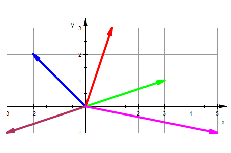
Für dickere Striche und Karos ist auch noch gesorgt.
-------------------------------------------------------------------------------------
Addition als Anhängen, Differen als Spitzenverbindung
av:=plot::Arrow2d(a,LineColor=RGB::Green):
bv:=plot::Arrow2d(b,LineColor=RGB::Blue):
bva:=plot::Arrow2d(a,a+b,LineColor=RGB::Blue,LineStyle=Dashed):
apb:=plot::Arrow2d(a+b,LineColor=RGB::Red):
ai:=plot::Arrow2d(-a,LineColor=RGB::Maroon):
amb:=plot::Arrow2d(b,a,LineColor=RGB::Magenta):
plot(av,bv,bva,apb,ai,amb, LineWidth=1,
Scaling=Constrained, GridVisible=TRUE)
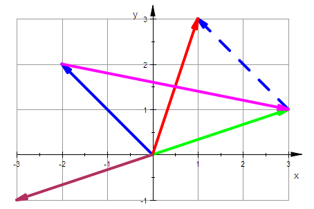
Ruft man also der Arrow2D-Befehl mit einem 2. Vektor auf,wird von
der Spitze des 1. Vektors zu Spitze des 2. Vektors ein Pfeil gezeichnet.
b an a angehängt realisiert man durch a,a+b
###############################################
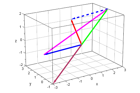
2. Vektoren 3D visualisieren
----------------------------------------------------------------------------------
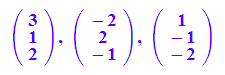
a := matrix([3,1,2]);
b := matrix([-2,2,-1]);


a,b,a+b,-a,a-b
av:=plot::Arrow3d(a,LineColor=RGB::Green):
bv:=plot::Arrow3d(b,LineColor=RGB::Blue):
bva:=plot::Arrow3d(a,a+b,LineColor=RGB::Blue,LineStyle=Dashed):
apb:=plot::Arrow3d(a+b,LineColor=RGB::Red):
ai:=plot::Arrow3d(-a,LineColor=RGB::Maroon):
amb:=plot::Arrow3d(b,a,LineColor=RGB::Magenta):
plot(av,bv,bva,apb,ai,amb, LineWidth=1,
Scaling=Constrained, GridVisible=TRUE)
#############################################
3. Vektorraumgesetze 3D visualisieren
----------------------------------------------------------------------------------
c := matrix([1,-1,-2]): a,b,c
----------------------------------------------------------------------------------
Assoziativgesetz
----------------------------------------------------------------------------------
a+(b+c)=(a+b)+c
av:=plot::Arrow3d(a,LineColor=RGB::Green):
bva:=plot::Arrow3d(a,a+b,LineColor=RGB::Blue):
apb:=plot::Arrow3d(a+b,LineColor=RGB::Magenta):
cv:=plot::Arrow3d(a+b,a+b+c,LineColor=RGB::Maroon):
bpc:=plot::Arrow3d(a,a+b+c,LineColor=RGB::Gray):
apbpc:=plot::Arrow3d(a+b+c,LineColor=RGB::Red):
plot(av,bva,apb,cv,bpc,apbpc, LineWidth=1,TipLength=8,
Scaling=Constrained, GridVisible=TRUE):
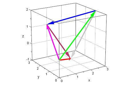
Doppelt anklicken, Drehen!!!!
Ursprung am Fuß von grün,rot,magenta
grün+blau+braun=rot
magenta + braun=rot
grün+grau=rot
----------------------------------------------------------------------------------
Distributivgesetz 1 r(a+b)=ra+rb
----------------------------------------------------------------------------------
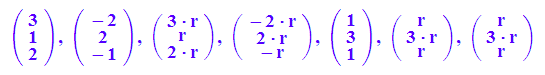
a,b,r*a,r*b,a+b,r*(a+b),r*a+r*b
r:=2:
av:=plot::Arrow3d(a,LineColor=RGB::Green):
bva:=plot::Arrow3d(a,a+b,LineColor=RGB::Blue):
apb:=plot::Arrow3d(a+b,LineColor=RGB::Magenta):
ra:=plot::Arrow3d(r*a,LineColor=RGB::Maroon,LineStyle=Dashed):
rbra:=plot::Arrow3d(r*a,r*a+r*b,LineColor=RGB::Black):
rapb:=plot::Arrow3d(r*(a+b),LineColor=RGB::Red,LineStyle=Dashed):
plot(av,bva,apb,ra,rbra,rapb, LineWidth=1,TipLength=8,
Scaling=Constrained, GridVisible=TRUE):
Doppelt anklicken, Drehen!!!!
Das Distributivgesetz 1 ist der Strahlensatz-Zusammenhang
##############################################
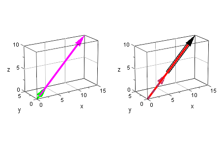
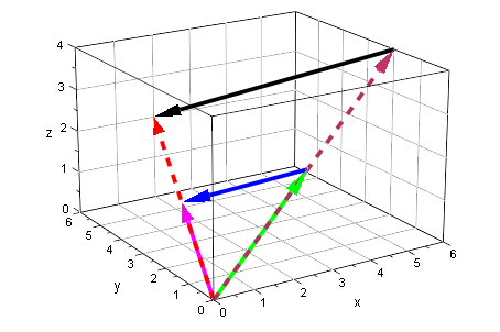
Distributivgesetz 2 
delete r,s:
a,r,s,(r+s)*a,r*a+s*a,r*a,s*a;
r:=2:s:=3:
av:=plot::Arrow3d(a,LineColor=RGB::Green,LineStyle=Dashed):
rpsa:=plot::Arrow3d((r+s)*a,LineColor=RGB::Magenta):
p1:=plot::Scene3d(av,rpsa,LineWidth=1,TipLength=8,
Scaling=Constrained, GridVisible=TRUE):
ra:=plot::Arrow3d(r*a,LineColor=RGB::Maroon,LineStyle=Dashed):
sa:=plot::Arrow3d(r*a,r*a+s*a,LineColor=RGB::Black,LineWidth=2):
rapsa:=plot::Arrow3d(r*a+s*a,LineColor=RGB::Red):
p2:=plot::Scene3d(rapsa,ra,sa, LineWidth=1,TipLength=8,
Scaling=Constrained, GridVisible=TRUE):
plot(p1,p2):