z:=x+I*y; w:=a+I*b
![]()
![]()
Komplexe Zahlen und Funktionen
unassume({a,b,x,y})
Dieses macht beim Wiederauswerten unten gemachte Annahmen rückgängig.
z:=x+I*y; w:=a+I*b
![]()
![]()
Definition von Komplexen Zahlen
z*w;expand(z*w); pe:=rectform(z*w)
![]()
![]()
![]()
Das Sortieren nach Real- und Imaginärteil kann natürlich nur klappen, wenn
man a,b,x,y,als reell ansieht:
assume(a,Type::Real): assume(b,Type::Real):
assume(x,Type::Real): assume(y,Type::Real):
Und nun nochmal
rectform(z*w)
![]()
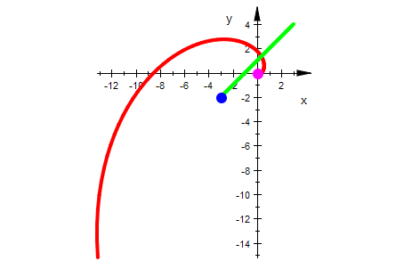
Komplexe Funktionen verbiegen das Koordinatengitter.
Darstellung der Quadratfunktion
//assume(x>0,Type::Real):
//assume(y>0,Type::Real):
rectform(z^2)
![]()
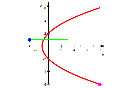
f:=(x,y)->[x^2-y^2 ,2*x*y];
![]()
P1:=plot::Point2d([x,1],x=-3..3, PointColor=[0,0,1]):
P1b:=plot::Point2d(f(x,y)|y=1,x=-3..3, PointColor=[1,0,1]):
Or:=plot::Point2d([0,0],x=-3..3):
oben1g:=plot::Curve2d([x,1],x=-3..3,LineColor=[0,1,0]):
f1g:=plot::Curve2d(f(x,y)|y=1,x=-3..3,LineColor=[1,0,0]):
plot(f1g,oben1g,P1,P1b,Scaling=Constrained,
PointSize=3, LineWidth=1)
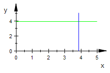
Sei also zuerst das Gitter im 1. Quadranten definiert:
waag:=[x,b]:senk:=[a,y]:
waagg:=plot::Curve2d(waag,x=0..5,b=0..5,LineColor=[0,1,0]):
senkg:=plot::Curve2d(senk,y=0..5,a=0..5):
plot(waagg,senkg)
:
waag:=[x,b]:senk:=[a,y]:
waagg:=plot::Curve2d(waag,x=-3..3,b=0..3,LineColor=[0,1,0]):
senkg:=plot::Curve2d(senk,y=-3..3,a=0..3):
biwaagg:=plot::Curve2d(f(x,b),x=-3..3,b=0..3,LineColor=[1,0,0]):
bisenkg:=plot::Curve2d(f(a,y),y=-3..3,a=0..3,LineColor=[1,0,1]):
plot(biwaagg,bisenkg,waagg,senkg,
Scaling=Constrained, LineWidth=0.7)
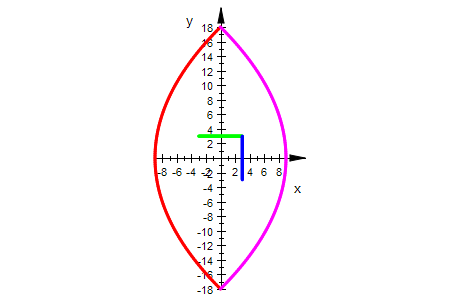
Der rote Bogen ist das Bild der grünen Strecke,
Der lila Bogen ist das Bild der blauen Strecke, bei der Quadratfunktion
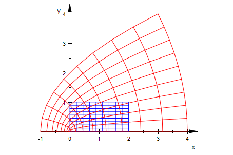
delete z:
ur:=plot::Conformal(z,z=0..2+I,Mesh=[10,10]):
bild:=plot::Conformal(z^2,z=0..2+I,Mesh=[10,10], LineColor=[1,0,0]):
plot(ur, bild,Scaling=Constrained)
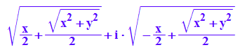
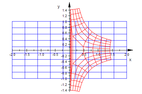
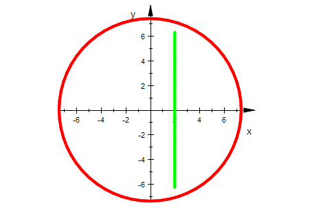
Darstellung der Wurzelfunktion
assume(x>0,Type::Real):
assume(y>0,Type::Real):
rectform(sqrt(x+I*y))
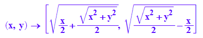
f:=(x,y)->[(1/2*x + 1/2*(x^2 + y^2)^(1/2))^(1/2) ,
(1/2*(x^2 + y^2)^(1/2) - 1/2*x)^(1/2)];
waag:=[x,b]:senk:=[a,y]:
waagg:=plot::Curve2d(waag,x=-5..5,b=0..5,LineColor=[0,1,0]):
senkg:=plot::Curve2d(senk,y=-5..5,a=0..5):
biwaagg:=plot::Curve2d(f(x,b),x=0..5,b=0..5,LineColor=[1,0,0]):
bisenkg:=plot::Curve2d(f(a,y),y=0..5,a=0..5,LineColor=[1,0,1]):
plot(biwaagg,bisenkg,waagg,senkg,
Scaling=Constrained)
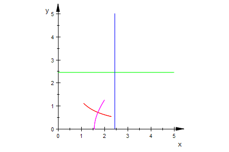
Der rote Bogen ist das Bild der grünen Strecke,
Der lila Bogen ist das Bild der blauen Strecke, bei der Wurzelfunktion
obeng:=plot::Curve2d([x,y],x=-3..3,y=0..3,LineColor=[1,0,0]):
unteng:=plot::Curve2d([x,y],x=-3..3,y=-3..0,LineColor=[1,0,0.5]):
riemannobg:=plot::Curve2d([x,y],x=-3..3,y=0..3,LineColor=[0,0,0.5]):
riemannuntg:=plot::Curve2d([x,y],x=-3..3,y=-3..0,LineColor=[0,1,0]):
f1q:=(x,y)->[(1/2*x + 1/2*(x^2 + y^2)^(1/2))^(1/2) ,
(1/2*(x^2 + y^2)^(1/2) - 1/2*x)^(1/2)];
f2q:=(x,y)->[-(1/2*x + 1/2*(x^2 + y^2)^(1/2))^(1/2) ,
(1/2*(x^2 + y^2)^(1/2) - 1/2*x)^(1/2)]:
f3q:=(x,y)->[-(1/2*x + 1/2*(x^2 + y^2)^(1/2))^(1/2) ,
-(1/2*(x^2 + y^2)^(1/2) - 1/2*x)^(1/2)]:
f4q:=(x,y)->[(1/2*x + 1/2*(x^2 + y^2)^(1/2))^(1/2) ,
-(1/2*(x^2 + y^2)^(1/2) - 1/2*x)^(1/2)]:

P1:=plot::Point2d([x,1],x=-3..3, PointColor=[0,0,1]):
P1b:=plot::Point2d(f1q(x,y)|y=1,x=-3..3, PointColor=[1,0,1]):
Or:=plot::Point2d([0,0],x=-3..3):
oben1g:=plot::Curve2d([x,1],x=-3..3,LineColor=[0,1,0]):
f11qg:=plot::Curve2d(f1q(x,y)|y=1,x=-3..3,LineColor=[1,0,0]):
plot(f11qg,Or,oben1g,P1,P1b,Scaling=Constrained,
PointSize=3, LineWidth=1)
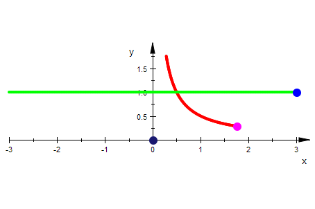
Waagerechte Gitterlinie und ihr Bild
delete z:
ur:=plot::Conformal(z,z=-2-I..2+I,Mesh=[10,10]):
bild:=plot::Conformal(sqrt(z),z=-2-I..2+I,Mesh=[10,10], LineColor=[1,0,0]):
plot(ur, bild,Scaling=Constrained)
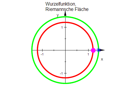
Polardarstellung und RiemannscheFläche
r:=1.44:
Pk1:=plot::Point2d([r*cos(t),r*sin(t)],t=0..4*PI,PointSize=4
,PointColor=[0,0,1], PointStyle=Stars):
Pk1b:=plot::Point2d([sqrt(r)*cos(t/2),sqrt(r)*sin(t/2)],t=0..4*PI
,PointSize=4,PointColor=[1,0,1]):
fg:=plot::Curve2d([sqrt(r)*cos(t/2),sqrt(r)*sin(t/2)],t=0..4*PI
,LineColor=[1,0,0], LineWidth=1):
urg:=plot::Curve2d([r*cos(t),r*sin(t)],t=0..2*PI,LineColor=[0,1,0]):
plot(fg, urg,Pk1,Pk1b,Scaling=Constrained, LineWidth=1
, TicksNumber=Low, Header="Wurzelfunktion,\nRiemannsche Fläche")
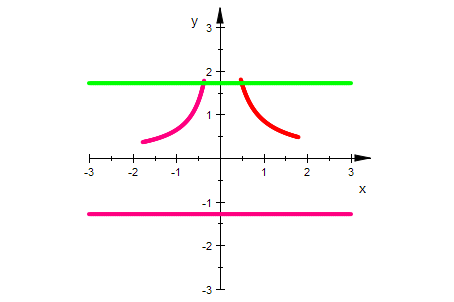
Waagerechte Gitterlinien und ihre Bilder
obeng:=plot::Curve2d([x,y],x=-3..3,y=0..3,LineColor=[0,1,0]):
f1qg:=plot::Curve2d(f1q(x,y),x=-3..3,y=0..3,LineColor=[1,0,0]):
f2qg:=plot::Curve2d(f2q(x,y),x=-3..3,y=-3..0,LineColor=[1,0,0.5]):
plot(f1qg,f2qg,obeng,unteng,LineWidth=1,Scaling=Constrained)
f3qg:=plot::Curve2d(f3q(x,y),x=-3..3,y=0..3,LineColor=[0,0,0.5]):
f4qg:=plot::Curve2d(f4q(x,y),x=-3..3,y=-3..0,LineColor=[0,1,0]):
plot(f3qg,f4qg,riemannobg,riemannuntg,
LineWidth=1,Scaling=Constrained)
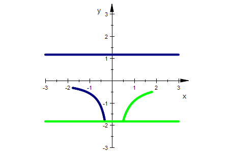
Man muss also zweimal mit den Waagerechten die Ebene übersteichen,
damit mann alle Bilder bekommt
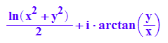
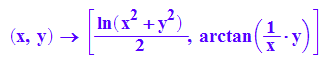
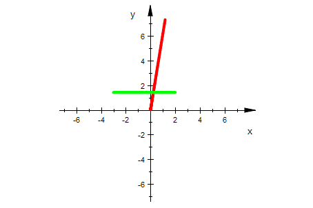
Darstellung der ln-Funktion
rectform(ln(z))
f:=(x,y)->[1/2*ln(x^2 + y^2) ,arctan(1/x*y)];
delete r:assume(r>0,Type::Real):assume(t,Type::Real):
Simplify(ln(r*E^(I*t)))
![]()
fpo:=(r,t)->[ln(r),t]
![]()
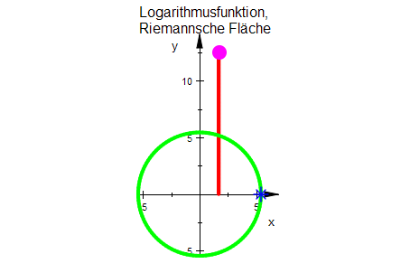
Die Darstellung in Polarkoordinaten ist passender.
r:=2*E:
Pk1:=plot::Point2d([r*cos(t),r*sin(t)],t=0..4*PI,PointSize=4
,PointColor=[0,0,1], PointStyle=Stars):
Pk1b:=plot::Point2d([ln(r),t],t=0..4*PI
,PointSize=4,PointColor=[1,0,1]):
fg:=plot::Curve2d([ln(r),t],t=0..4*PI
,LineColor=[1,0,0], LineWidth=1):
urg:=plot::Curve2d([r*cos(t),r*sin(t)],t=0..2*PI,LineColor=[0,1,0]):
plot(fg, urg,Pk1,Pk1b,Scaling=Constrained, LineWidth=1
, TicksNumber=Low, Header="Logarithmusfunktion,\nRiemannsche Fläche")
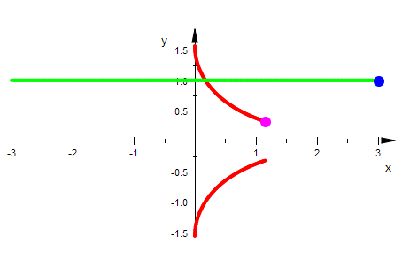
P1:=plot::Point2d([x,1],x=-3..3, PointColor=[0,0,1]):
P1b:=plot::Point2d(f(x,y)|y=1,x=-3..3, PointColor=[1,0,1]):
Or:=plot::Point2d([0,0],x=-3..3):
oben1g:=plot::Curve2d([x,1],x=-3..3,LineColor=[0,1,0]):
f1g:=plot::Curve2d(f(x,y)|y=1,x=-3..3,LineColor=[1,0,0]):
plot(f1g,oben1g,P1,P1b,Scaling=Constrained,
PointSize=3, LineWidth=1)
Darstellung der Exponentialfunktion
E^z
![]()
f:=(x,y)->[E^x*cos(y),E^x*sin(y)]
![]()
P1:=plot::Point2d([x,1],x=-3..3, PointColor=[0,0,1]):
P1b:=plot::Point2d(f(x,y)|y=1,x=-3..3, PointColor=[1,0,1]):
Or:=plot::Point2d([0,0],x=-3..3):
oben1g:=plot::Curve2d([x,1],x=-3..3,LineColor=[0,1,0]):
f1g:=plot::Curve2d(f(x,y)|y=1,x=-3..3,LineColor=[1,0,0]):
plot(f1g,oben1g,P1,P1b,Scaling=Constrained,
PointSize=3, LineWidth=1)
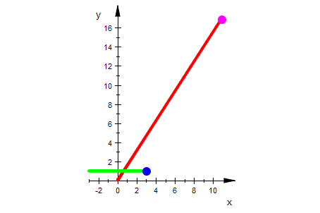
Die waagerechten Geraden werden auf Strahlen vom Ursprung aus abgebildet.
Dabei haben Waagrerechte Geraden mit dem Abstand 2 PI denselben Strahl als Bild.
P1:=plot::Point2d([1,y],y=-2*PI..3*PI, PointColor=[0,0,1]):
P1b:=plot::Point2d(f(x,y)|x=1,y=-2*PI..3*PI, PointColor=[1,0,1]):
Or:=plot::Point2d([0,0],x=-3..3):
senk1g:=plot::Curve2d([1,y],y=-2*PI..3*PI,LineColor=[0,1,0]):
f1g:=plot::Curve2d(f(x,y)|x=1,y=-2*PI..3*PI,LineColor=[1,0,0]):
plot(f1g,senk1g,P1,P1b,Scaling=Constrained,
PointSize=3, LineWidth=1)
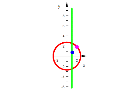
Die senkrechten Geraden werden auf Kreise um den Ursprung abgebildet.
Dabei werden Punkte mit dem senkrechten Abstand 2 PI auf denselbenPunkt abgebildet.
Die ganze Ebene ist Urbild und die ganze Ebene ist Bild
f(x,y)
![]()
oben1g:=plot::Curve2d([x,y],x=-3..2,y=-2*PI..2*PI,LineColor=[0,1,0]):
f1g:=plot::Curve2d(f(x,y),x=-3..2,y=-2*PI..2*PI,LineColor=[1,0,0]):
plot(f1g,oben1g,Scaling=Constrained,
PointSize=3, LineWidth=1)
ur:=plot::Conformal(z,z=0..1+2*PI*I,Mesh=[10,10]):
bild:=plot::Conformal(E^z,z=0..1+2*PI*I,Mesh=[40,40], LineColor=[1,0,0]):
plot(ur, bild,Scaling=Constrained)
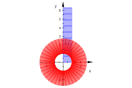
Die waagerechten Geraden werden auf Strahlen vom Ursprung aus abgebildet.
Dabei haben Waagrerechte Geraden mit dem Abstand 2 PI denselben Strahl als Bild.
senk1g:=plot::Curve2d([x,y],y=-2*PI..2*PI,x=-3..2,LineColor=[0,1,0]):
f1g:=plot::Curve2d(f(x,y),y=-2*PI..2*PI,x=-3..2,LineColor=[1,0,0]):
plot(f1g,senk1g,Scaling=Constrained,
PointSize=3, LineWidth=1)
Die senkrechten Geraden werden auf Kreise um den Ursprung abgebildet.
Dabei werden Punkte mit dem senkrechten Abstand 2 PI auf denselbenPunkt abgebildet.
Die ganze Ebene ist Urbild und die ganze Ebene ist Bild
P1:=plot::Point2d([x,1+x],x=-3..3, PointColor=[0,0,1]):
P1b:=plot::Point2d(f(x,y)|y=1+x,x=-3..3, PointColor=[1,0,1]):
Or:=plot::Point2d([0,0],x=-3..3):
oben1g:=plot::Curve2d([x,1+x],x=-3..3,LineColor=[0,1,0]):
f1g:=plot::Curve2d(f(x,y)|y=1+x,x=-3..3,LineColor=[1,0,0]):
plot(f1g,oben1g,P1,P1b,Scaling=Constrained,
PointSize=3, LineWidth=1)
Beliebige Geraden werden auf Spiralen abgebildet.