Prof. Dr. Dörte Haftendorn Ha /02
In[737]:=
![f[x_] := Cos[1/x] ; f[0] = 0 ; f '[x] f[h]/h (* Differenzenquotient für x = 0 *) f ''[x] ... 1}, {x, -3, 3}, PlotStyle -> farbig, PlotRange -> {-1, 1.5}, AspectRatio -> Automatic] ;](coswunder_2.gif)
Out[738]=
![]()
Out[739]=
![]()
Out[740]=
![]()
![[Graphics:coswunder_6.gif]](coswunder_6.gif)
In[742]:=
![Limit[f[x], x -> 0] (* nicht stetig in x = 0 *) Limit[f '[x], x -> 0] Limit[f[h]/h, h -> 0] (* Differenzialquotient für x = 0 ex . nicht *)](coswunder_7.gif)
Out[742]=
![]()
Out[743]=
![]()
Out[744]=
![]()
In[745]:=
![h[x_] := x Cos[1/x] h '[x] h[k]/k (* Differenzenquotient für x = 0 *) h ''[x] hGraph = Pl ... x}, {x, -2, 2}, PlotStyle -> farbig, PlotRange -> {-1, 1.5}, AspectRatio -> Automatic] ;](coswunder_11.gif)
Out[746]=
![]()
Out[747]=
![]()
Out[748]=
![[Graphics:coswunder_15.gif]](coswunder_15.gif)
In[750]:=
![Limit[h[x], x -> 0] Limit[h '[x], x -> 0] Limit[h[k]/k, k -> 0] (* Differenzialquotient für x = 0 ex . nicht *) Limit[h ' '[x], x -> 0]](coswunder_16.gif)
Out[750]=
![]()
Out[751]=
![]()
Out[752]=
![]()
Out[753]=
![]()
In[754]:=
![]()
In[755]:=
![]()
Out[755]=
![]()
In[756]:=
![]()
Out[756]=
![]()
In[757]:=
![hhAsyGraph = Plot[{h[x], x, x}, {x, -3, 2}, PlotStyle -> farbig, PlotRange -> {-1, 2}, AspectRatio -> Automatic] ;](coswunder_28.gif)
![[Graphics:coswunder_29.gif]](coswunder_29.gif)
In[758]:=
![Limit[h[x] - x, x -> ∞] (* Asymptote y = x *) Limit[h '[x] - 1, x -> ∞] Limit[h ''[x], x -> ∞]](coswunder_30.gif)
Out[758]=
![]()
Out[759]=
![]()
Out[760]=
![]()
In[761]:=
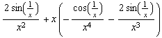
![hh[x_] := x^2 Cos[1/x] hh '[x] hh[h]/h (* Differenzenquotient für x = 0 *) hh ''[x]](coswunder_34.gif)
Out[762]=
![]()
Out[763]=
![]()
Out[764]=
In[765]:=
![hhGraph = Plot[{hh[x], x^2, -x^2}, {x, -2, 2}, PlotStyle -> farbig, PlotRange -> {-1, 1}, AspectRatio -> Automatic] ;](coswunder_38.gif)
![[Graphics:coswunder_39.gif]](coswunder_39.gif)
In[766]:=
![Limit[hh[x], x -> 0] Limit[hh '[x], x -> 0] (* nicht stetig in x = 0 *) Limit[hh[h]/h, h -> 0] (* Differenzialquotient für x = 0 ex . *) Limit[hh ' '[x], x -> 0]](coswunder_40.gif)
Out[766]=
![]()
Out[767]=
![]()
Out[768]=
![]()
Out[769]=
![]()
In[770]:=
![]()
In[771]:=
![]()
Out[771]=
![]()
In[772]:=
![]()
Out[772]=
![]()
In[773]:=
![hhAsyGraph = Plot[{hh[x], x^2, x^2 - 1/2}, {x, -3, 2}, PlotStyle -> farbig, PlotRange -> {-1, 2}, AspectRatio -> Automatic] ;](coswunder_52.gif)
![[Graphics:coswunder_53.gif]](coswunder_53.gif)
In[774]:=
![Limit[hh[x] - x^2 + 1/2, x -> ∞] (* Asymptote y = x^2 - 1/2 *) Limit[hhh '[x] - 2 x, x -> ∞] Limit[hhh ''[x] - 2, x -> ∞]](coswunder_54.gif)
Out[774]=
![]()
Out[775]=
![]()
Out[776]=
![]()
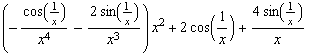
In[777]:=
![hhh[x_] := x^3 Cos[1/x] hhh '[x] hhh[h]/h (* Differenzenquotient für x = 0 *) hhh ''[x]](coswunder_58.gif)
Out[778]=
![]()
Out[779]=
![]()
Out[780]=
In[781]:=
![hhhGraph = Plot[{hhh[x], x^3, -x^3}, {x, -.1, .1}, PlotStyle -> farbig (* , PlotRange -> {-0.1, 1}, AspectRatio -> Automatic *)] ;](coswunder_62.gif)
![[Graphics:coswunder_63.gif]](coswunder_63.gif)
In[782]:=
![Limit[hhh[x], x -> 0] Limit[hhh '[x], x -> 0] (* stetig in x = 0 *) Limit[hhh[h]/h, h -& ... ferenzialquotient für x = 0 *) Limit[hhh ' '[x], x -> 0] (* Unbeschränkt in x = 0 *)](coswunder_64.gif)
Out[782]=
![]()
Out[783]=
![]()
Out[784]=
![]()
Out[785]=
![]()
In[786]:=
![]()
In[787]:=
![]()
Out[787]=
![]()
In[788]:=
![]()
Out[788]=
![]()
In[789]:=
![hhhAsyGraph = Plot[{hhh[x], x^3, -x^3, x^3 - 1/2 x}, {x, -1, 2}, PlotStyle -> farbig, PlotRange -> {-1/2, 2}, AspectRatio -> Automatic] ;](coswunder_76.gif)
![[Graphics:coswunder_77.gif]](coswunder_77.gif)
In[790]:=
![Limit[hhh[x] - x^3 + 1/2 x, x -> ∞] (* Asymptote y = x^3 - 1/2 x *) Limit[hhh '[x] - 3 x^2 + 1/2, x -> ∞] Limit[hhh ''[x] - 6 x, x -> ∞]](coswunder_78.gif)
Out[790]=
![]()
Out[791]=
![]()
Out[792]=
![]()
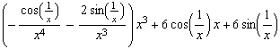
In[793]:=
![hhhh[x_] := x^4 Cos[1/x] hhhh '[x] hhhh[h]/h (* Differenzenquotient für x = 0 *) hhhh ''[x]](coswunder_82.gif)
Out[794]=
![]()
Out[795]=
![]()
Out[796]=
In[797]:=
![hhhhGraph = Plot[{hhhh[x], x^4, -x^4}, {x, -.1, .1}, PlotStyle -> farbig (* , PlotRange -> {-0.1, 1}, AspectRatio -> Automatic *)] ;](coswunder_86.gif)
![[Graphics:coswunder_87.gif]](coswunder_87.gif)
In[798]:=
![Limit[hhhh[x], x -> 0] Limit[hhhh '[x], x -> 0] Limit[hhhh[h]/h, h -> 0] (* Differenzialquotient für x = 0 *) Limit[hhhh ' '[x], x -> 0]](coswunder_88.gif)
Out[798]=
![]()
Out[799]=
![]()
Out[800]=
![]()
Out[801]=
![]()
In[802]:=
![]()
In[825]:=
![]()
Out[825]=
![]()
In[826]:=
![]()
Out[826]=
![]()
In[805]:=
![hhhAsyGraph = Plot[{hhhh[x], x^3, -x^3, asyyyy}, {x, -0.7, 0.7}, PlotStyle -> farbig, PlotRange -> {-0.05, 0.1}] ;](coswunder_100.gif)
![[Graphics:coswunder_101.gif]](coswunder_101.gif)
In[806]:=
![Limit[hhhh[x] - asyyyy, x -> ∞] (* Asymptote y = x^4 - 1/2 x^2 + 1/24 *) Limit[hhhh '[x] - 4 x^3 + x, x -> ∞] Limit[hhhh ''[x] - 12 x^2 + 1, x -> ∞]](coswunder_102.gif)
Out[806]=
![]()
Out[807]=
![]()
Out[808]=
![]()
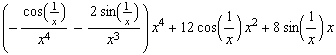
In[809]:=
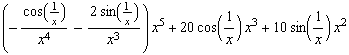
![hhhhh[x_] := x^5 Cos[1/x] hhhhh '[x] hhhhh[h]/h (* Differenzenquotient für x = 0 *) hhhhh ''[x] <br />](coswunder_106.gif)
Out[810]=
![]()
Out[811]=
![]()
Out[812]=
In[813]:=
![hhhhhGraph = Plot[{hhhhh[x], x^5, -x^5}, {x, -.1, .1}, PlotStyle -> farbig (* , PlotRange -> {-0.1, 1}, AspectRatio -> Automatic *)] ;](coswunder_110.gif)
![[Graphics:coswunder_111.gif]](coswunder_111.gif)
In[814]:=
![Limit[hhhhh[x], x -> 0] Limit[hhhhh '[x], x -> 0] Limit[hhhhh[h]/h, h -> 0] (* Differenzialquotient für x = 0 *) Limit[hhhhh ' '[x], x -> 0]](coswunder_112.gif)
Out[814]=
![]()
Out[815]=
![]()
Out[816]=
![]()
Out[817]=
![]()
In[818]:=
![]()
In[827]:=
![]()
Out[827]=
![]()
In[828]:=
![]()
Out[828]=
![]()
In[821]:=
![hhhAsyGraph = Plot[{hhhhh[x], x^3, -x^3, asyyyyy}, {x, -0.7, 0.7}, PlotStyle -> farbig, PlotRange -> {-0.05, 0.1}] ;](coswunder_124.gif)
![[Graphics:coswunder_125.gif]](coswunder_125.gif)
In[822]:=
![Limit[hhhhh[x] - asyyyyy, x -> ∞] (* Asymptote y = x^5 - 1/2 x^3 + 1/24 x *) Limit[hh ... [x] - 5 x^4 + 3/2 x^2 - 1/24, x -> ∞] Limit[hhhhh ''[x] - 20 x^3 + 3 x, x -> ∞]](coswunder_126.gif)
Out[822]=
![]()
Out[823]=
![]()
Out[824]=
![]()
Converted by Mathematica (July 27, 2003)