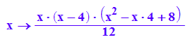
fff1:=x->x*(x-4); fff2:=x->(x-2)^2; fff3:=x->(x-2)^2+3;
![]()
![]()
![]()
Polynome 4.Grades vollständig
Prof. Dr. Dörte Haftendorn MuPAD 4 April 07 https://mathe.web.leuphana.de
#####################################################################
Die Ableitungen der Polynome 4. Grades sind Polynome vom Grad 2.
Damit kommen i.w. nur die folgenden drei Typen infrage.
Die an der x-Achse gespiegelten Versionen werden nicht gesondert betrachtet.
fff1:=x->x*(x-4); fff2:=x->(x-2)^2; fff3:=x->(x-2)^2+3;
![]()
![]()
![]()
plotfunc2d(fff1,fff2,fff3,ViewingBoxYRange=-4..10)
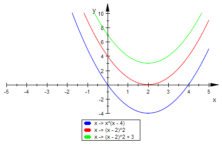
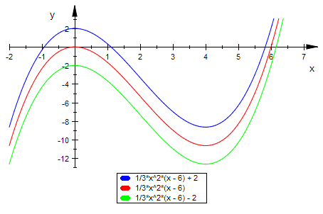
Typ 1: f'' hat zwei Nullstellen
Durch Integration ergibt sich eine Stammfunktion, die drei typische Lagen haben kann.
ff11:=x-->int(fff1(x), x): ff11(x);
ff10:=x-->ff11(x)+2;
ff12:=x-->ff11(x)-2;
plotfunc2d(ff10(x),ff11(x),ff12(x),x=-2..7,ViewingBoxYRange=-13..3)

Typ 2: f '' hat eine doppelte Nullstelle
Durch Integration ergibt sich eine Stammfunktion, die zwei typische Lagen haben kann.
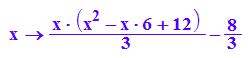
ff21:=x-->int(fff2(x), x): ff21(x);
ff21(2)

![]()
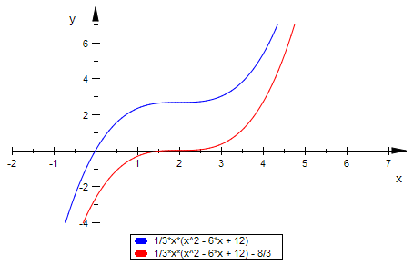
ff22:=x-->ff21(x)-8/3;
plotfunc2d(ff21(x),ff22(x),x=-2..7,ViewingBoxYRange=-4..7)
Typ 3: f '' hat keine Nullstelle
Durch Integration ergibt sich eine Stammfunktion, die zwei typische Lagen haben kann.
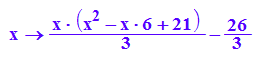
ff31:=x-->int(fff3(x), x): ff31(x);
ff31(2)

![]()
ff32:=x-->ff31(x)-26/3;
plotfunc2d(ff31(x),ff32(x),x=-2..7,ViewingBoxYRange=-3..16)

Im Folgenden werden die zugehörigen Formtypen für f,
das Polynom 4. Grades ermittelt und weiter unten gezeichnet.
Typ 1: f hat zwei Wendepunkte
f10:=x-->int(ff10(x), x);
//plotfunc2d(f10,x=-2..9,ViewingBoxYRange=-25..8)

f11:=x-->int(ff11(x), x);
//plotfunc2d(f11,x=-2..9,ViewingBoxYRange=-40..10)

f12:=x-->int(ff12(x), x);
//plotfunc2d(0.5*f12,x=-2..9,ViewingBoxYRange=-25..8)

Typ 2: f hat eine "starke Plattstelle"
f21:=x-->int(ff21(x), x);
//plotfunc2d(f21,x=-2..7,ViewingBoxYRange=-2..12)

f22:=x-->int(ff22(x), x);
//plotfunc2d(f22,x=-2..7,ViewingBoxYRange=-2..12)
Typ 3: f hat eine "schwache Plattstelle", "Beulenstelle"
f31:=x-->int(ff31(x), x);
//plotfunc2d(0.3*f31,x=-2..6,ViewingBoxYRange=-8..12)
f32:=x-->int(ff32(x), x);
//plotfunc2d(0.3*f32,x=-2..6,ViewingBoxYRange=-8..12)
Zeichnungen für alle vorkommenden Typen von
Polynomen 4. Grades.
2. Ableitung ist gepunktet, 1. Ableitung ist gestrichelt, f selbst ist durchgezogen.
fff1p:=plot::Function2d(fff1(x),x=-2..6,ViewingBoxYRange=-5..2,
LineColor=[0,0,1], LineStyle=Dotted, LineWidth=1.4):
fff2p:=plot::Function2d(fff2(x),x=-2..6,ViewingBoxYRange=-5..2,
LineColor=[1,0,0], LineStyle=Dotted, LineWidth=1.4):
fff3p:=plot::Function2d(fff3(x),x=-2..6,ViewingBoxYRange=-5..6,
LineColor=[0,1,0], LineStyle=Dotted, LineWidth=1.4):
plot(fff1p,fff2p,fff3p)

Typ 1: f '' hat zwei Nullstellen, f hat zwei Wendepunkte
ff10p:=plot::Function2d(ff10(x),x=-2..6,ViewingBoxYRange=-8..6,
LineColor=[0,0,0], LineStyle=Dashed, LineWidth=0.8):
ff11p:=plot::Function2d(ff11(x),x=-2..6,ViewingBoxYRange=-11..2,
LineColor=[1,0,0], LineStyle=Dashed, LineWidth=0.8):
ff12p:=plot::Function2d(ff12(x),x=-2..6,ViewingBoxYRange=-13..2,
LineColor=[0,1,0], LineStyle=Dashed, LineWidth=0.8):
plot(fff1p,ff10p,ff11p,ff12p)

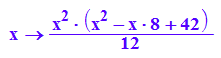
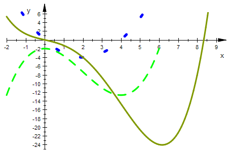
Typ 10 f hat drei Extremstellen, f' drei einfache Nullstellen
f10p:=plot::Function2d(0.35*f10(x),x=-2..9,ViewingBoxYRange=-13..6,
LineColor=[1,0,1], LineWidth=0.8):
plot(fff1p,ff10p,f10p)
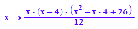
Typ 11 f hat eine Sattelstelle und eine Extremstelle
f' eine doppelte und eine einfach Nullstelle
f11p:=plot::Function2d(0.35*f11(x),x=-2..9,ViewingBoxYRange=-13..6,
LineColor=[0,0.5,1], LineWidth=0.8):
plot(fff1p,ff11p,f11p)
Typ 12 f hat einen schrägen Sattel und ein Extremum.
f ' genau eine einfache Nullstelle
f12p:=plot::Function2d(0.5*f12(x),x=-2..9,ViewingBoxYRange=-25..6,
LineColor=[0.5,0.6,0], LineWidth=0.8):
plot(fff1p,ff12p,f12p)
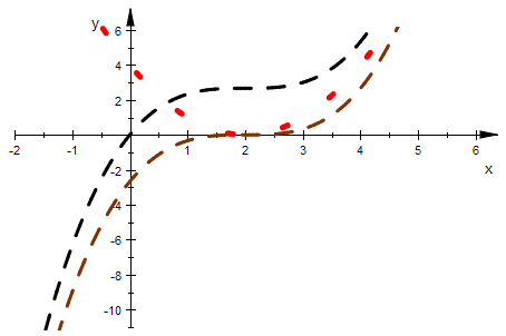
Typ 2 f '' hat eine doppelte Nullstelle, f ' hat einen Sattel,
f hat keinen Wendepunkt
ff21p:=plot::Function2d(ff21(x),x=-2..6,ViewingBoxYRange=-8..6,
LineColor=[0,0,0], LineStyle=Dashed, LineWidth=0.8):
ff22p:=plot::Function2d(ff22(x),x=-2..6,ViewingBoxYRange=-11..2,
LineColor=[0.5,0.2,0], LineStyle=Dashed, LineWidth=0.8):
plot(fff2p,ff21p,ff22p)
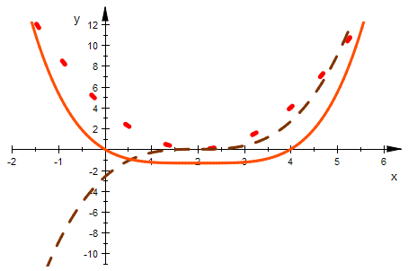
Typ 21 f hat eine starke Plattstelle und eine Extremstelle
f ' einen Sattel und eine einfache Nullstelle
f21p:=plot::Function2d(f21(x),x=-2..6,ViewingBoxYRange=-2..12,
LineColor=[0.3,0.3,0.3], LineWidth=0.8):
plot(fff2p,ff21p,f21p)

Typ 22 f hat breites Extremum.
f ' eine dreifache Nullstelle
f22p:=plot::Function2d(f22(x),x=-2..6,ViewingBoxYRange=-2..12,
LineColor=[1,0.3,0], LineWidth=0.8):
plot(fff2p,ff22p,f22p)
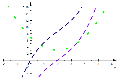
Typ 3 f '' hat keine Nullstelle, f ' hat einen schrägen Sattel und eine
einfache Nullstelle, f hat ein einfaches Extremum
ff31p:=plot::Function2d(ff31(x),x=-2..6,ViewingBoxYRange=-2..16,
LineColor=[0,0,0.5], LineStyle=Dashed, LineWidth=0.8):
ff32p:=plot::Function2d(ff32(x),x=-2..6,ViewingBoxYRange=-2..16,
LineColor=[0.5,0,1], LineStyle=Dashed, LineWidth=0.8):
plot(fff3p,ff31p,ff32p)
Typ 31: f hat eine einfaches Extremum und eine "Beule"
f31p:=plot::Function2d(0.3*f31(x),x=-2..6,ViewingBoxYRange=-2..12,
LineColor=[0.3,0.3,0], LineWidth=0.8):
plot(fff3p,ff31p,f31p)

Typ 32: f hat eine einfaches Extremum das zugleich eine "Beule" ist.
f32p:=plot::Function2d(f32(x),x=-2..6,ViewingBoxYRange=-8..12,
LineColor=[1,0,1], LineWidth=0.8):
plot(fff3p,ff32p,f32p)
