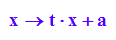
p1:=x->t*x+a;
p2:=x->m*(x-x1)+p1(x1);
p3:=x->n*(x-x2)+p2(x2);
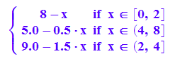
f:=x->piecewise([0<=x and x<=x1,p1(x)],
[x1<x and x<=x2,p2(x)],
[x2<x and x<=x3,p3(x)]):


Ökonomie, Zusammengesetzte Funktionen
Prof. Dr. Dörte Haftendorn, MuPAD 4, Dez.06 Update Jan 07
Web: https://mathe.web.leuphana.de www.mathematik-verstehen.de
+++++++++++++++++++++++++++++++++++++++++++++++++++++++++++++++++++++
p1:=x->t*x+a;
p2:=x->m*(x-x1)+p1(x1);
p3:=x->n*(x-x2)+p2(x2);
f:=x->piecewise([0<=x and x<=x1,p1(x)],
[x1<x and x<=x2,p2(x)],
[x2<x and x<=x3,p3(x)]):
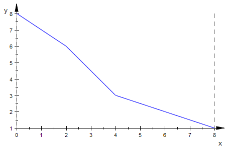
a:=8: t:=-1: m:=-1.5: n:=-0.5: x1:=2: x2:=4:x3:=8:
plotfunc2d(f(x),x=0..x3)
f(x)
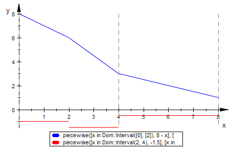
Zeichnung mit den Ableitungen:
plotfunc2d(f(x), f'(x),x=0..x3);
Daraus wird gebildet:
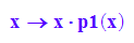
g1(x):=x->x*p1(x);
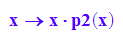
g2(x):=x->x*p2(x);
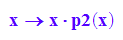
g3(x):=x->x*p2(x);
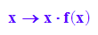
g(x):=x->x*f(x);
Dazu kommt noch die Gerade h
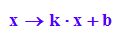
h:=x->k*x+b;
k:=1: b:=3:
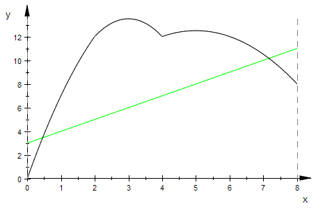
Um die Integralflächen zu zeichnen, muss man Graphikojekte erzeugen:
fpl:=plot::Function2d(f(x),x=0..x3);
gpl:=plot::Function2d(g(x),x=0..x3, LineColor=[0,0,0]);
hpl:=plot::Function2d(h(x),x=0..x3, LineColor=[0,1,0]);
plot(hpl,gpl);



zwisch:=plot::Hatch(gpl,hpl,x=0..x3):
plot(zwisch,gpl,hpl)
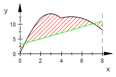
Hier ist zuviel genommen.
Nun sind die Schnittpunkte von g und h zu bestimmen
solve(g(x)=h(x),x)
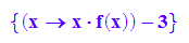
Das geht so nicht, also einzeln
xs:=solve(x*p1(x)=h(x),x)
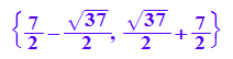
Davon nehmen wir den ersten Wert
xsl:=xs[1]

Ebenso
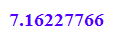
xs:=solve(x*p3(x)=h(x),x);
xsr:=xs[2];

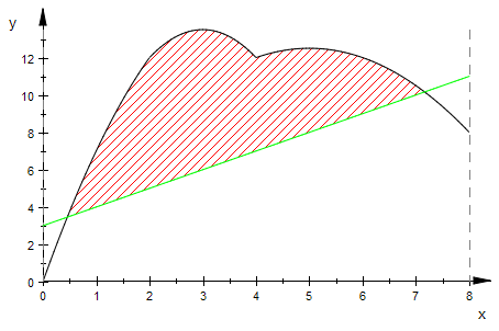
gplz:=plot::Function2d(g(x),x=xsl..xsr, LineColor=[0,0,0]);
hplz:=plot::Function2d(h(x),x=xsl..xsr, LineColor=[0,1,0]);
zwisch:=plot::Hatch(gplz,hplz,x=xsl..xsr):
plot(zwisch,gpl,hpl)


Berechnung des Integrals
int(g(x)-h(x), x=xsl..xsr)
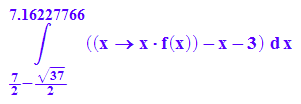
Geht so nicht. Also einzeln
i1:=float(int(x*p1(x)-h(x), x=xsl..x1));
i2:=int(x*p2(x)-h(x), x=x1..x2);
i3:=int(x*p3(x)-h(x), x=x2..xsr);
i1+i2+i3
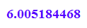

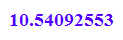

Die letzte Zahl ist die Gesamtfläche.