datenPunkte:=[1,5], [2,2],[5,3],[7,5]:
dp:=datenPunkte;
![]()
Lagrange- Interpolationspolynom
Prof. Dr. Dörte Haftendorn, MuPAD 4, http://haftendorn.uni-lueneburg.de Aug.06
Automatische Übersetzung aus MuPAD 3.11, Nov. 05 Update Juni 06
Es fehlen noch textliche Änderungen, die MuPAD 4 direkt berücksichtigen, das ist in Arbeit.
Web: http://haftendorn.uni-lueneburg.de www.mathematik-verstehen.de
+++++++++++++++++++++++++++++++++++++++++++++++++++++++++++++++++++++
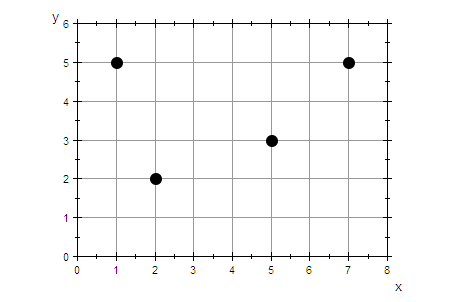
Konstruiert für 4 Datenpunkte, die hier beliebig eingeben werden können.
Eine Anpassung der Zeichenbereiche ist ggf. dann "von Hand" nötig".
datenPunkte:=[1,5], [2,2],[5,3],[7,5]:
dp:=datenPunkte;
![]()
Gesucht ist ein Polynom durch die 4 Datenpunkte.
graphDatenPunkte:=plot::Listplot([datenPunkte],
LinesVisible=FALSE, PointSize=3,Scaling=Constrained,
GridVisible=TRUE,ViewingBox=[0..8,0..6]):
plot(graphDatenPunkte)
Basis-Polynome nach Lagrange
Idee: Es werden Polynome aus 3 Linearfaktoren konstruiert, die an
genau 3 der 4 Stützstellen ihre Nullstellen haben.
Sie sind eine Basis im Polynomraum der Polynome bis zuum 3. Grad.
Die gesuchte Lösung p ist damit eine Linearkombination dieser 4 Polynome
dp
![]()
L0:=x->(x-dp[2][1])*(x-dp[3][1])*(x-dp[4][1]): L0(x);
L1:=x->(x-dp[1][1])*(x-dp[3][1])*(x-dp[4][1]): L1(x);
L2:=x->(x-dp[1][1])*(x-dp[2][1])*(x-dp[4][1]): L2(x);
L3:=x->(x-dp[1][1])*(x-dp[2][1])*(x-dp[3][1]): L3(x);
![]()
![]()
![]()
![]()
p:=x->c0*L0(x)+c1*L1(x)+c2*L2(x)+c3*L3(x);p(x)
![]()
![]()
c0:=dp[1][2]/L0(dp[1][1]);
c1:=dp[2][2]/L1(dp[2][1]);
c2:=dp[3][2]/L2(dp[3][1]);
c3:=dp[4][2]/L3(dp[4][1]);
![]()
![]()
![]()
![]()
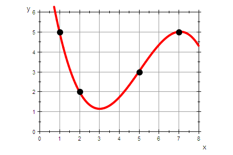
p(x)

graphp:=plot::Function2d(p(x),x=0..8,
LineColor=RGB::Red, LineWidth=1):
plot(graphp,graphDatenPunkte)
gL0:=plot::Function2d(L0(x),x=0..8,
LineColor=RGB::Black, LineWidth=1):
gL1:=plot::Function2d(L1(x),x=0..8,
LineColor=RGB::Blue, LineWidth=1):
gL2:=plot::Function2d(L2(x),x=0..8,
LineColor=RGB::Magenta, LineWidth=1):
gL3:=plot::Function2d(L3(x),x=0..8,
LineColor=RGB::Green, LineWidth=1):
xA:=plot::Function2d(0,x=0..8,
LineColor=RGB::DarkGray, LineWidth=1):
plot(xA,gL0,gL1,gL2,gL3,graphp,graphDatenPunkte,
ViewingBox=[0..8,-7..9], Scaling=Unconstrained)
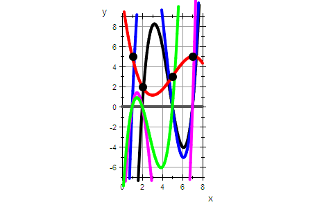
Hier sieht man also die 4 Basispolynome, die also an genau 3
Stützstellen ihre Nullstellen haben.
Es gibt nur ein einziges Polynom minimalen Grades durch die Datenpunkte.
Mit jeder Methode ergibt sicg dasselbe Polynom.
####################################################
Interpolationspolynom direkt von MuPAD
Zuerst müssen die Datenpunkte in einer x-Datenliste und einer
y-Datenliste aufgenommen werden.
xd:=[dp[i][1]$i=1..4];
yd:=[dp[i][2]$i=1..4];
![]()
![]()
ip:=interpolate(xd,yd,x)

Das Interpolationspolynom ist vom Datentyp "Polynom".
es kann an jeder Stelle ausgewertet werden, wie eine Funktion.
ip(3)
![]()
gripol:=plot::Function2d(ip(x),x=0..8,
LineColor=[0.8,0,0.8], LineWidth=1, LineStyle=Dashed):
plot(graphp,gripol,graphDatenPunkte,
ViewingBox=[0..8,-2..6])
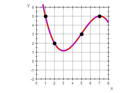
Es passt natürlich aufeinander.
################################################