f:=x->x+cos(x);
![]()
Numerische Analysis x+cos(x)
Prof. Dr. Dörte Haftendorn: Mathematik mit MuPAD 4, Update Mai 07
exsistiert auch als MuPAD 3-Version Aug. 05
www.uni-lueneburg.de/mathe-lehramt http:haftendorn.uni-lueneburg.de
---------------------------------------------------------------------------------------------------------
1. Aus Bausteinen aufbauen, Nullstelle berechnen
2. Funktion näherungsweise Integrieren ( Fläche)
3. Funktion näherungsweise Integrieren( Rotationsvolumen)
#########################################################
f:=x->x+cos(x);
![]()
plotfunc2d(x,x+cos(x),cos(x))
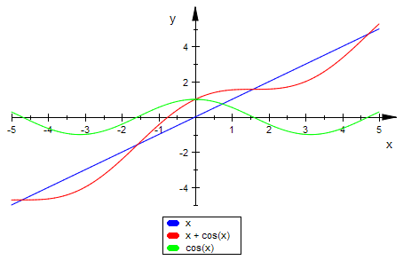
Ersichtlich liegt nur eine Nullstelle vor.
Bestimmung mit MuPAD
xs:=numeric::solve(f(x)=0,x)[1];
![]()
Bestimmung mit Newtonverfahren
f'(x)
![]()
newt:=x->x-f(x)/f'(x)
x0:=-1.0:
[x0,f(x0),f'(x0),f(x0)/f'(x0),newt(x0)]
![]()
Hier sind die Werte, die man von Hand braucht.
Mehrfache Anwendung des Newtonverfahrens:
(newt @@ k)(x0) $k=1..4
![]()
Das wird stabil, also ist der Startwert gut.
2. Funktion näherungsweise Integrieren
Beispiel: Berechnen Sie Fläche unter f im Bereich zwischen der Nullstelle und x=3.
re:=3.0:mi:=(xs+re)/2;
![]()
[re-xs, f(xs),f(mi),f(re)];
kl:=[(re-xs)/6, f(xs),4*f(mi),f(re)]
![]()
![]()
Berechnung nach der Kepler-Regel
kepWert:=kl[1]*(kl[2]+kl[3]+kl[4]);
![]()
zum Vergleich mit Integration
int(f(x),x=xs..re);
![]()
Vergelich mit einem Rechteck Breite 4 Höhe 1.6 (aus Graphen)
R:=4*1.6
![]()
Das passt.
2. Funktion näherungsweise Integrieren
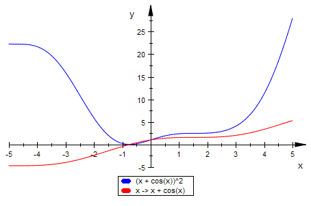
Beispiel: Berechnen Sie das Rotationsvolumen von f um die
x-Achse im Bereich zwischen der Nullstelle und x=3.
f:=x->x+cos(x)
![]()
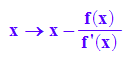
fq ist die Funktion, die bei einem Volumenproblem mit f(x)=x+ cos(x) auftritt.
fq:=x->(x+cos(x))^2
![]()
plotfunc2d(fq(x),f)
xs:=numeric::solve(f(x)=0,x)[1];
re:=3.0;
![]()
![]()
vase:=plot::XRotate(f(x),x=xs..re): plot(vase)
mi:=(xs+re)/2
![]()
fg:=plot::Function2d(f(x),x=-2..4, LineStyle=Dashed):
fqg:=plot::Function2d(fq(x),x=-2..4, LineColor=[1,0,0]):
ende:=plot::Line2d([re,fq(re)],[re,0]):
mitte:=plot::Line2d([mi,fq(mi)],[mi,0]):
plot(fg,fqg, ende, mitte)
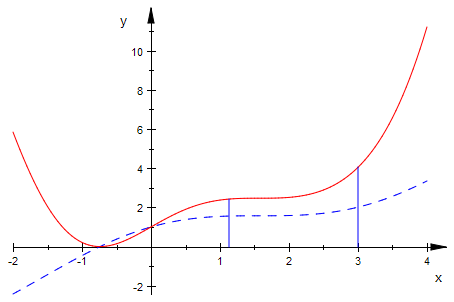
[re-xs, fq(xs),fq(mi),fq(re)];
kl:=[(re-xs)/6, fq(xs),4*fq(mi),fq(re)]
![]()
![]()
Berechnung nach der Kepler-Regel
kepWert:=PI*kl[1]*(kl[2]+kl[3]+kl[4]);
float(kepWert)
![]()
![]()
zum Vergleich mit Integration
PI*int(fq(x),x=xs..re);
float(%)
![]()
![]()
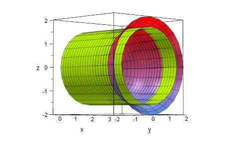
Vergleichszylinder, Radius dem Graphen entnommen
r:=1.6: Vz:=PI*r^2*(3-xs)
![]()
Das passt.
zy:=plot::XRotate(1.6,x=xs..3)
![]()
plot(vase,zy)
##########################################